In May of 2025, GDAL, opens in a new tab (the Geospatial Data Abstraction Library) released version 3.11, opens in a new tab of their ubiquitous raster (and vector) processing library and related tools.
As part of their focus on the CLI experience in this release, they introduced raster pipelines. Raster pipelines, opens in a new tab are a way to chain together most CLI commands into one expression. Think of it like Unix pipes for GDAL commands, but using ! instead of |. Each step is calculated on-the-fly without writing anything to disk until the final output step (unless specifically instructed to do so at an earlier stage).
This has two big advantages that I can see (discovering others is left as an exercise for the readers):
- No more littering your working directory with intermediate datasets that clog up your file listings (and eat your storage)
- Saving a pipeline in its serialized .gdalg.json, opens in a new tab format allows you to use the result of the entire processing chain as the input to other GDAL utilities now or in the future, just as if it were any other raster data type, without actually creating a new dataset on disk.
The first point is a great quality of life improvement. It smooths off a lot of the friction of working with the GDAL CLI (along with the other CLI improvements in 3.11).
Saving the pipeline as a serialized algorithm is similar to GDAL’s VRT virtual raster format. Where I use VRTs to mosaic together a bunch of tiles into a single large raster without having to write the resulting file to disk, pipelines allow me to save a set of processes without writing the final (or intermediate) output to disk. When I load the pipeline, everything is done on the fly.
Let’s Fill the Pipe
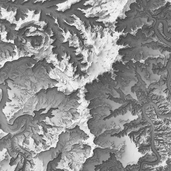
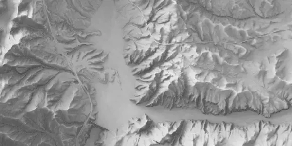
I recently created a new version of our statewide skyshade using the latest 10 meter DEMs from the USGS that (for the most part) have been updated from the 3DEP Lidar program. To save processing time, I ran my skyshade program, opens in a new tab on a 30 meter downsampled version of the DEMs (we’d lose some detail, but the output of the skyshade is supposed to be nice soft and fuzzy shadows anyways).
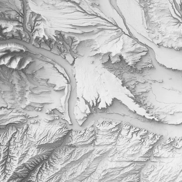
I want to process the 30 meter, float32-based output skyshade to a 10 meter, byte-based raster. Scaling the values down to bytes will also require re-assigning a valid nodata value. I want to convert to byte because the outputs of the skyshade all fall within 0-255 with a bunch of extra precision that’s not needed when the display is going to be an 8-bit grayscale color ramp. Using bytes shrinks the resulting file to 25% the size of the float32 original.
Here’s what that pipeline looks like:
gdal raster pipeline ! read 30m_all_turbid-315-15-250-200steps.tif ! scale --ot byte --dst-min=1 --dst-max=255 ! resize --resolution 10,10 -r cubic ! edit --nodata 0 ! write --co compress=lzw --co bigtiff=yes 30m_skyshade_10m-2.tifBreaking it Down into Byte-Sized Pieces
This command has five discrete steps:
read: This is the starting point for standard processing pipelines and accesses the source raster.scale: Converts the data values from their current float32 range down to 1-255. The--ot byteparameter converts the values to byte-based ints. I leave 0 available for nodata.resize: Changes the resolution down to 10 meters by 10 meters (I’m using a meter-based CRS here). The default nearest-neighbor resampling looks ugly and can introduce unexpected artifacts so I specify cubic resampling with-r cubic.edit: My source raster has a nodata of -999999, which gets moved up to 0 when converting to byte-based ints. We need to flag this as the new nodata value to hide these areas along the edges (which resulted from projecting the lat/long source DEM data into UTM 12N NAD83)write: Now that the data should be looking right, the final step writes it out to disk, or “materializes” it. I’m using the common--cocreation options flag to compress the resulting data for even more storage savings.
And that’s all there is to it. In about 5 minutes of runtime I’ve got my new rescaled, resized raster all ready to go.